II. Logistic regression
0. Presentation
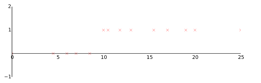
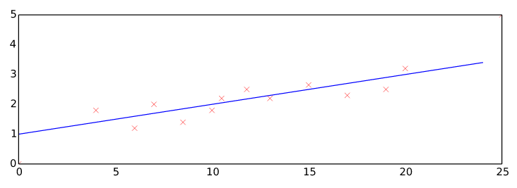
Idea: classify y=0 (negative class) or y=1 (positive class)
From linear regression hθ(x)=θTX We need to choose hypothesis function such as 0≤h(x)≤1
1. Hypothesis function
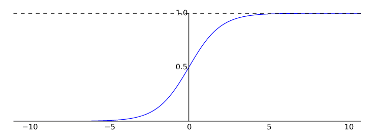
hθ(x)=g(i=0∑nθixi)forg(z)=1+e−z1
Notes: Octave implementation of sigmoid function
g = 1 ./ ( 1 + e .^ (-z));
Vectorized form:
Since ∑i=0nθixi=θTX. The vectorized form of hθ(x) is
1+e−θTX1orsigmoid(θTX)
Octave implementation
h = sigmoid(theta' * X)
h(x) is the estimate probability that y=1 on input x
When sigmoid(θTX)≥0.5 then we decide y=1. As we know sigmoid(θTX)≥0.5 when θTX≥0
So for y=1 , θTX≥0. We call θTX is the line that define the Decision boundary that separate the area where y=0 and y=1. It does not need to be linear since X can contain polynomial term.
Decision boundary is the property of the hypothesis and parameter θ, not of the training set
2. The cost function
We need to choose the cost function so that it is “convex” toward one single global minimum
Cost function
J(θ)=m1i=1∑mCost(hθ(x(i),y(i)))withCost(hθ(x(i),y(i)))={−log(hθ(x))−log(1−hθ(x))ifify=1y=0
A simplified form of the cost function is:
J(θ)=−m1[i=1∑my(i)log(hθ(x(i))+(1−y(i))log(1−hθ(x(i)))]
Vectorized form:
J(θ)=m1(−yTlog(sigmoid(Xθ))−(1−yT)log(1−sigmoid(Xθ)))
Code in Octave to compute cost function
J = (1/m) * ( -y' * log(sigmoid(X*theta) ) - (1-y') * log(1-sigmoid(X*theta)) );
We need to get the parameter θ where J(θ) is min. Then we can make a prediction when given new x using
hθ(x)=1+e−θTX1
3. Gradient Descent algorithm
Using Gradient Descent to find value of θ when J(θ) is min, we have
Repeat until convergence
θj:=θj−α∂θj∂J(θ)
Repeat until convergence
θj:=θj−αm1i=1∑m(hθ(x(i))−y(i))x(i)
Vectorized form:
θ:=θ−mα(XT(sigmoid(Xθ)−y⃗))
Code in Octave to compute gradient step ∂θj∂J(θ)
grad = (1 / m) * (X' * (sigmoid( X * theta) - y) );
4. Adding Regularization parameter
Regularized cost function:
J(θ)=−m1[i=1∑my(i)log(hθ(x(i))+(1−y(i))log(1−hθ(x(i)))]+2mλj=1∑nθj2
The second sum, ∑j=1nθj2 means to explicitly exclude the bias term, θ0. I.e. the θ vector is indexed from 0 to n (holding n+1 values, θ0 through θn), and this sum explicitly skips θ0, by running from 1 to n, skipping 0.
Octave code to compute cost function with regularization
J = (1/m) * (-y' * log(sigmoid(X*theta)) - (1-y')*log(1-sigmoid(X*theta))) + lambda/(2*m)*sum(theta(2:end).^2);
Thus, when computing the equation, we should continuously update the two following equations:
Regularized Gradient Descent:
Repeat
{
θ0θj:=θ0−αm1i=1∑m(hθ(x(i))−y(i))x0(i):=θj−α[(m1i=1∑m(hθ(x(i))−y(i))x(i))+mλθj]forj≥1
}
Octave code to compute gradient step ∂θj∂J(θ)
grad = (1 / m) * (X' * (sigmoid( X * theta) - y)) + (lambda/m)*[0; theta(2:end)];
Notice that we don’t add the regularization term for θ0
5. Advanced Optimization
Prepare a function that can compute J(θ) and ∂θj∂J(θ) for a given θ
function [jVal, gradient] = costFunction(theta)
  jVal = [...code to compute J(theta)...];
  gradient = [...code to compute derivative of J(theta)...];
end
Then with this function Octave can provide us some advanced algorithms to compute min of J(θ). We should not implement these below algorithms by ourselves.
- Conjugate gradient
- BFGS
- L-BFGS
options = optimset('GradObj', 'on', 'MaxIter', 100);
initialTheta = zeros(2,1);
[optTheta, functionVal, exitFlag] = fminunc(@costFunction, initialTheta, options);
We give to the function fminunc() our cost function, our initial vector of theta values, and the options object that we created beforehand.
Advantages:
No need to pick up α.
Often faster than gradient descent.
Disadvantages:
More complex.
Practical advice: try a couple of different libraries.