Machine Learning class note 2 - Linear Regression

I. Linear regression

0. Presentation

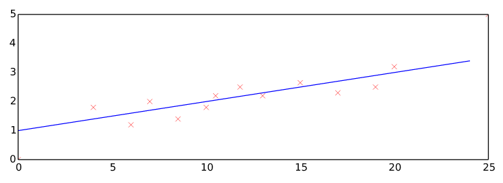
Idea: try to fit the best line to the training sets

1. Hypothesis function

$\begin{array}{cc}{h}_{\theta }\left(x\right)& ={\theta }_0+{\theta }_1{x}_1+{\theta }_2{x}_2+\mathrm{.}\mathrm{.}\mathrm{.}\\ & ={\sum }_{i=0}^n{\theta }_i{x}_i\end{array}$
\begin{aligned}
h_\theta(x) & = \theta_0 + \theta_1x_1 + \theta_2x2 + … \
& = \sum{i=0}^{n}\theta_ixi
\end{aligned}

Vectorized form:
$h_{\theta }\left(x\right)=\left[\begin{array}{cccc}{\theta }_0& {\theta }_1& {\theta }_2& \mathrm{.}\mathrm{.}\mathrm{.}\end{array}\right]\left[\begin{array}{c}{x}_0\\ x_1\\ x_2\\ \mathrm{.}\mathrm{.}\mathrm{.}\end{array}\right]={\theta }^{T}X$
h\theta(x) = \left[\begin{matrix} \theta_0 & \theta_1 & \theta_2 & … \end{matrix}\right] \left[\begin{matrix} x_0 \ x_1 \ x_2 \ … \end{matrix}\right] = \theta^TX

Octave implemtation
Prepping by adding an all-one-column in front of X for $x_0$

h = theta' * X

The line fits best when the distance of our hypothesis to the sample training set is minimum.

Distance from hypothesis to the training set $h_\theta(x) -y = \theta_0 + \theta_1x_1 + \theta_2x_2 + … - y$

2. The cost function

Do the above for every sample point we arrive at the cost function below (or square error function or mean squared error)

$J_{\left(\theta \right)}=\frac{1}{2m}{\sum }_{i=1}^m{\left(h_{\theta }\right(x^{\left(i\right)})-y^{\left(i\right)})}^2$
J{(\theta)} = \frac{1}{2m}\sum{i=1}^{m} \left( h_\theta ( x^{(i)} ) - y^{(i)} \right) ^ 2

Octave implementation

J = 1 / (2*m) * sum((X * theta - y).^2)

Vectorized form:

$J_{\left(\theta \right)}=\frac{1}{2m}(X\theta -\vec{y}{)}^T(X\theta -\vec{y})$
J_{(\theta)} = \frac{1}{2m}(X\theta - \vec{y}) ^ T ( X\theta - \vec{y})

J = 1 / (2*m) * (X*theta - y)' * (X*theta - y);

3. Batch Gradient Descent algorithm

To find out the value of $\theta$ when $J_{(\theta)}$ is min, we can use batch Gradient descent rule below:

Repeat until convergence
${\theta }_j:={\theta }_j-\alpha \frac{\mathrm{\partial }}{\mathrm{\partial }{\theta }_j}J\left(\theta \right)$
\theta_j := \theta_j - \alpha \frac {\partial }{\partial \theta_j}J(\theta)

and if we take the partial derivative of $J_{(\theta)}$ respect to $\theta_j$ we have:
Repeat until convergence
${\theta }_j:={\theta }_j-\alpha \frac{1}{m}{\sum }_{i=1}^m\left(h_{\theta }\right(x^{\left(i\right)})-y^{\left(i\right)})x^{\left(i\right)}$
\theta_j := \thetaj - \alpha \frac{1}{m} \sum{i=1}^{m} \left( h_\theta ( x^{(i)} ) - y^{(i)} \right) x^{\left(i\right)}

Octave implementation

for feature = 1:size(X, 2)
  theta(feature) = theta(feature) - alpha*(1/m) * sum((X*theta-y) .* X(:,feature));
end

Vectorized form:
$\theta :=\theta -\frac{\alpha }{m}\left(X^T\right(X\theta -\vec{y}\left)\right)$
\theta := \theta - \frac{\alpha}{m} \left( X^T (X\theta - \vec{y}) \right)

Octave implementation

theta = theta - alpha*(1/m) * (X' * (X*theta-y));

Notes on using gradient descent

Gradient descent need many iteration and works well for number of features n > 10,000

Complexity of $O(n^2)$

Choosing alpha:
Should step 0.1, 0.3, 0.6, 1 …

Feature normalization
To make gradient descent converges faster we can normalize the data a bit
$x_i=\frac{x_i-{\mu }_i}{s_i}$
x_i = \frac{x_i - \mu_i}{s_i}

where mu_i is the average of all the value of feature i
s_i is the range of value or the standard deviation of feature i

After having theta, we can plug X and theta back in hypothesis function to find out the prediction
$h_\theta(x) = \theta^TX$

4. Adding Regularization parameter

Why Regularization ?
The more features introduced, the higher chances that overfitting happens. To address overfitting, we can reduce the number of features or use regularization:

• Keep all the features, but reduce the magnitude of parameters θj.
• Regularization works well when we have a lot of slightly useful features.

How? Adding regularization parameter changing:

Regularized cost function:
$J_{\left(\theta \right)}=\frac{1}{2m}[{\sum }_{i=1}^m{\left(h_{\theta }\right(x^{\left(i\right)})-y^{\left(i\right)})}^2+\lambda {\sum }_{j=1}^n{\theta }_j^2]$
J{(\theta)} = \frac{1}{2m} \left [ \sum{i=1}^{m} \left( h\theta ( x^{(i)} ) - y^{(i)} \right) ^ 2 + \lambda \sum{j=1}^{n}\theta_j^2 \right]

Regularized Gradient Descent:

We will modify our gradient descent function to separate out $\theta_0$ from the rest of the parameters because we do not want to penalize $\theta_0$.

Repeat
{
$\begin{array}{cc}{\theta }_0& :={\theta }_0-\alpha \frac{1}{m}{\sum }_{i=1}^m\left(h_{\theta }\right(x^{\left(i\right)})-y^{\left(i\right)})x_0^{\left(i\right)}\\ {\theta }_j& :={\theta }_j-\alpha [\left(\frac{1}{m}{\sum }_{i=1}^m\left(h_{\theta }\right(x^{\left(i\right)})-y^{\left(i\right)})x^{\left(i\right)}\right)+\frac{\lambda }{m}{\theta }_j]\text{<mi mathvariant="normal">f</mi><mi mathvariant="normal">o</mi><mi mathvariant="normal">r</mi>}j\ge 1\end{array}$
\begin{aligned}
\theta_0 &:= \theta0 - \alpha \frac{1}{m} \sum{i=1}^{m} \left( h_\theta ( x^{(i)} ) - y^{(i)} \right) x_0^{\left(i\right)} \
\theta_j &:= \thetaj - \alpha \left[ \left( \frac{1}{m} \sum{i=1}^{m} \left( h_\theta ( x^{(i)} ) - y^{(i)} \right) x^{\left(i\right)} \right) + \frac{\lambda}{m}\theta_j \right] \quad \textrm{for} \quad j \geq 1
\end{aligned}

}

5. Normal equation

There is another way to minimize $J_{(\theta)}$. This is the explicitly way to compute value of $\theta$ without resorting to an iterative algorithm.
$\theta =(X^{T}X{)}^{-1}{X}^T\vec{y}$
\theta = (X^TX)^{-1} X^T\vec{y}

Sometimes $(X^TX)$ is non-invertable. Some of the reasons include existence of redundant features or too many features $(m \leq n)$. We should recude number of feature or switch to gradient descent in such case.

Octave implementation

theta = (X' * X)^(-1) * X' * y;

Notes on using Normal equation

No need to choose alpha.

No need to run many iterations.

Feature scaling is also not necessary.

Complexity of $O(n^3)$ since we need to calculate inverse of $(X^TX)$ or pinv(X'* X)

Close of n is very large, should switch to gradient descent.

We can also apply regularization to the normal equation
$\begin{array}{cc}& \theta =(X^{T}X+\lambda \cdot L{)}^{-1}{X}^T\vec{y}\\ & \text{<mi mathvariant="normal">w</mi><mi mathvariant="normal">i</mi><mi mathvariant="normal">t</mi><mi mathvariant="normal">h</mi>}L=\left[\begin{array}{ccccc}0& & & & \\ & 1& & & \\ & & 1& & \\ & & & \ddots & \\ & & & & 1\end{array}\right]\end{array}$
\begin{aligned}
&\theta = (X^TX+ \lambda \cdot L)^{-1} X^T\vec{y} \
&\textrm{with} \quad L = \begin{bmatrix}
0 & & & &\
& 1 & & & \
& & 1 & & \
& & & \ddots & \
& & & & 1
\end{bmatrix}
\end{aligned}

Recall that if $m < n$, and may be non-invertible if $m = n$ then $X^TX$ is non-invertible. However, when we add the term $\lambda \cdot L$, then $X^TX + \lambda \cdot L$ becomes invertible.